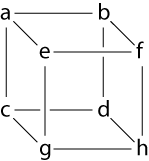
 | edge(a, b) edge(a, c) edge(c, d) edge(b, d) edge(a, e) edge(b, f) | edge(c, g) edge(d, h) edge(e, f) edge(e, g) edge(g, h) edge(f, h) | vertex(a) vertex(b) vertex(c) vertex(d) vertex(e) vertex(f) vertex(g) vertex(h) |
We'll collect this set of facts and call the collection of propositions (20 atomic propositions in all) GRAPH.
Also not terribly interesting, but maybe ever-so-slightly interesting, is that one can take this representation of a graph and do forward-chaining logic programming with it. Consider, for example, the following forward-chaining logic program made up of two rules.
edge(Y,X) <- edge(X,Y).These are just logical propositions; the upper-case identifiers are implicitly universally quantified, the comma represents conjunction, and (following common convention for logic programming) we write implication backwards as B <- A instead of A -> B. We'll call this collection of two rules REACH.
reachable(Y) <- edge(X,Y), reachable(X), vertex(Y).
Recall that the behavior of a forward chaining logic program is to take facts that it has and learn more facts. If we just throw the graph at this program, it will use the first rule to derive all the backwards edges (edge(b,a), edge(c,a), and so on) but nothing else. If we add an additional single fact reachable(a), then our forward chaining logic program will furiously learn that b, c, and indeed all the other vertices are reachable. We can rephrase this in the following way: for a specific choice of X and Y, there is a path from X to Y if and only if there is a derivation of this sequent:
GRAPH, REACH ⊢ reachable(X) -> reachable(Y)In fact, the forward chaining logic programming engine, given reachable(X) for some specific X, will derive a fact of the form reachable(Y) for every reachable Y.
Twist 1: weighted logic programming
The first interesting twist on our boring program is this: we consider those proofs of the sequentGRAPH, REACH ⊢ reachable(X) -> reachable(Y)and we ask, what if some proofs are better than others? One way to introduce a metric for "what is better" is to say that every one of those atomic propositions has a cost, and every time we use that atomic proposition in a proof we have to pay that cost: we want the cheapest proof:
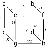 | edge(a, b) = 66 edge(a, c) = 53 edge(c, d) = 12 edge(b, d) = 57 edge(a, e) = 19 edge(b, f) = 53 | edge(c, g) = 92 edge(d, h) = 6 edge(e, f) = 8 edge(e, g) = 84 edge(g, h) = 162 edge(f, h) = 4 | vertex(a) = 0 vertex(b) = 0 vertex(c) = 0 vertex(d) = 0 vertex(e) = 0 vertex(f) = 0 vertex(g) = 0 vertex(h) = 0 |
Related work
In fact we can play the same game on any semiring as long as the "score" of a proof is the semiring product of the score of the axioms (in this case, "plus" was the semiring product) and the way we combine the scores of different proofs is the semiring sum of the scores of the two proofs (in this case, "min" was the semiring sum). This sort of generalization-to-an-arbitrary semiring is something that isn't noticed as much as it probably should be. If you're interested in learning or thinking more about weighted logic programming, the first eleven pages of the paper I coauthored with Shay Cohen and Noah Smith, Products of Weighted Logic Programs, were written specifically as a general audience/programming languages audience introduction to weighted logic programming. Most of the other literature on weighted logic programming is by Jason Eisner, though the semiring generalization trick was first extensively covered by Goodman in the paper Semiring Parsing; that paper was part of what inspired Eisner's work on weighted logic programming, at least as I understand it.Twist 2: linear logic programming
Another direction that we can "twist" this initially graph discussion is by adding linearity. Linear facts (in the sense of linear logic) are unlike "regular" facts - regular facts can be used any number of times or used not at all - they are persistent. Linear facts can only be used once in a proof - and in fact, they must be used once in a proof.We've had the vertex propositions hanging around all this time and not doing much; one thing we can do is make these vertex propositions linear, and we'll make the reachable propositions linear as well. In this example, we'll designate linear propositions by underlining them and coloring them red; our program before turns into this:
edge(Y,X) <- edge(X,Y).By the way, if you're familiar with linear logic, the logical meaning of this formula is captured by the following two propositions written properly in linear logic:
reachable(Y) <- edge(X,Y), reachable(X), vertex(Y).
∀x. ∀y. !edge(x,y) -o edge(y,x).We'll talk a little bit more about this specification (call it LREACH) shortly; for the moment let's switch to a different train of thought.
∀x. ∀y. !edge(x,y) -o reachable(x) -o vertex(y) -o reachable(y).
Greedy logic programming with linear logic
When we talked before about the cost of using a fact in a proof, we were actually assuming a little bit about proofs being focused; we'll talk a little bit about focusing and synthetic rules in this section (see this old blog post for background).If we make all of our atomic propositions positive, then the synthetic rule associated with the critical second rule above ends up looking like this:
Γ, edge(X,Y); Δ, reachable(Y) ⊢ CRecall that we like to read forward chaining rules from the bottom to the top. If we assume that the context only ever contains a single reachable(X) proposition, then we can think of the linear context as a resource consuming automaton that is in state X. At each step, the automaton consumes an available resource vertex(Y) with the constraint that there must be an edge from X to Y; the automaton then transitions to state Y.
---------------------------------------------
Γ, edge(X,Y); Δ, reachable(X), vertex(Y) ⊢ C
One efficient way to give a logic programming semantics to these kind of forward-chaining linear logical specifications is to just implement an arbitrary run of the automaton without ever backtracking. This is a greedy strategy, and it can be used to efficiently implement some greedy algorithms. This was the point of Linear Logical Algorithms, a paper I coauthored with Frank Pfenning. One neat example from that paper was the following graph program, which computes a spanning tree for a graph rooted at the vertex a:
edge(Y,X) <- edge(X,Y).This program works like another little resource-consuming automaton that, at each step, consumes a vertex resource to add a non-tree vertex to the tree along a newly added tree edge. This is, incidentally, the same way Prim's algorithm for minimum spanning trees progresses.
intree(a) <- vertex(a).
tree(X,Y), intree(Y) <- edge(X, Y), intree(X), vertex(Y).
Hamiltonian paths in linear logic
The greedy strategy where we look at one possible set of choices is very different than the behavior of our briefly-sketched forward-chaining persistent and weighted logic programming engines. The latter worked by taking some initial information (reachable(X) for some X) and finding, all at once and with reasonable efficiency, every single Y for a given X such that the following sequent holds:GRAPH, REACH ⊢ reachable(X) -> reachable(Y)Call the (persistent) edges EDGE, and the (linear) vertices VERT. Now we can look at the (seemingly) analogous problem stated in linear logic to see why it is in practice, so different:
LREACH, EDGE; VERT ⊢ ⊢ reachable(X) -o reachable(Y)Because linear logic requires that we eventually use every resource in VERT, this derivation corresponds to a run of the automaton where the automaton visited every single node and then ended at Y. If we consider just the case where X and Y are the same, complete derivations correspond to Hamiltonian tours.
By adding linearity, we've made the forward chaining language more expressive, but in doing so we created a big gulf between the "existential" behavior (here's one way the automaton might work, which we found by being greedy) and the "universal" behavior (the automaton can, potentially, follow a Hamiltonian path, which we learned by calling a SAT solver). This gap did not exist, at least for our running example, in the persistent or weighted cases.
Combining the twists?
Both linear logic programming and weighted logic programming arise start from a simple observation: the shape of proofs can capture interesting structures. The "structure" in this case was a path through a graph; in weighted logic programming the structures are often parse trees - you know, "boy" is a noun, "fast" is an adverb, "the" is a demonstrative adjective, and the two combined are a noun phrase, until you get a tree that looks something like this:Sentence(More on this in the "Products of Weighted Logic Programs" paper.)
/ \
NP VP
/| | \
/ | | \
D N V A
| | | |
the boy ran fast
Weighted logic programming enriches this observation by allowing us to measure structures and talk about the combined measure of a whole class of structures; linear logic, on the other hand, greatly improves on the things that we can measure. But what about using the observations of weighted logic programming to assign scores in the richer language of linear logic programming? What would that look like? I'll give a couple of sketches. These are questions I don't know the answers to, don't know that I'll have time to think about in the near future, but would love to talk further about with anybody who was interested.
Minimum spanning tree
I commented before that the logic programming engine described in Linear Logical Algorithms implements something a bit like Prim's algorithm to produce a graph spanning tree. In fact, the engine we described does so with provably optimal complexity - O(|E| + |V|), time proportional to the number of edges in the graph or the number of vertices in the graph (whichever is larger). What's more, we have a good cost semantics for this class of weighted logic programs; this means you don't actually have to understand how the interpreter works, you can reason about the runtime behavior of linear logical algorithms on a much more abstract level. The recorded presentation on Linear Logical Algorithms, as well as the paper, discuss this.If we replace a queue inside the engine with an appropriately configured priority queue, then the logic programming engine actually implements Prim's algorithm for the low cost of an log(|V|) factor. But can this be directly expressed as a synthesis of weighted logic programming and linear logic programming? And can we do so while still maintaining a reasonable cost semantics? I don't know.
Traveling salesman problem
While minimum spanning tree is a greedy "existential" behavior of linear logic proof search, the weighted analogue of the Hamiltonian Path problem is just the Traveling Salesman problem - we not only want a Hamiltonian path, we want the best Hamiltonian path as measured by a straightforward extension of the notion of weight from weighted logic programming.Not-linear logics?
Adding some linearity turned a single-source shortest path problem into a Hamiltonian path problem - when we turned vertices from persistent facts into linear resources, we essentially required each vertex to be "visited" exactly once. However, an affine logic interpretation of the same program would preserve the resource interpretation (vertices cannot be revisited) while removing the obligation - vertices can be visited once or they can be ignored altogether.This makes the problem much more like the shortest path problem again. If edge weights are positive, then the shortest path never revisits a node, so it's for all intents and purposes exactly the shortest path problem again. If edge weights are negative, then disallowing re-visiting is arguably the only sensible way to specify the problem at all. Can this observation be generalized? Might it be possible to solve problems in (weighted) affine logic more easily than problems in weighted linear logic?

